MGC
-
class
hyppo.independence.MGC(compute_distance='euclidean', **kwargs)¶ Multiscale Graph Correlation (MGC) test statistic and p-value.
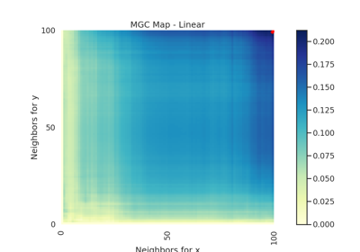
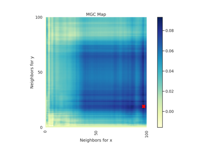
Specifically, for each point, MGC finds the \(k\)-nearest neighbors for one property (e.g. cloud density), and the \(l\)-nearest neighbors for the other property (e.g. grass wetness) [1]. This pair \((k, l)\) is called the "scale". A priori, however, it is not know which scales will be most informative. So, MGC computes all distance pairs, and then efficiently computes the distance correlations for all scales. The local correlations illustrate which scales are relatively informative about the relationship. The key, therefore, to successfully discover and decipher relationships between disparate data modalities is to adaptively determine which scales are the most informative, and the geometric implication for the most informative scales. Doing so not only provides an estimate of whether the modalities are related, but also provides insight into how the determination was made. This is especially important in high-dimensional data, where simple visualizations do not reveal relationships to the unaided human eye. Characterizations of this implementation in particular have been derived from and benchmarked within in [2]. A description of the process of MGC and applications on neuroscience data can be found in [1]. It is performed using the following steps:
Let \(x\) and \(y\) be \((n, p)\) samples of random variables \(X\) and \(Y\). Let \(D^x\) be the \(n \times n\) distance matrix of \(x\) and \(D^y\) be the \(n \times n\) be the distance matrix of \(y\). \(D^x\) and \(D^y\) are modified to be mean zero columnwise. This results in two \(n \times n\) distance matrices \(A\) and \(B\) (the centering and unbiased modification) [3].
For all values \(k\) and \(l\) from \(1, ..., n\),
The \(k\)-nearest neighbor and \(l\)-nearest neighbor graphs are calculated for each property. Here, \(G_k (i, j)\) indicates the \(k\)-smallest values of the \(i\)-th row of \(A\) and \(H_l (i, j)\) indicates the \(l\) smallested values of the \(i\)-th row of \(B\)
The local correlations are summed and normalized using the following statistic:
\[c^{kl} = \frac{\sum_{ij} A G_k B H_l} {\sqrt{\sum_{ij} A^2 G_k \times \sum_{ij} B^2 H_l}}\]
The MGC test statistic is the smoothed optimal local correlation of \(\{ c^{kl} \}\). Denote the smoothing operation as \(R(\cdot)\) (which essentially set all isolated large correlations) as 0 and connected large correlations the same as before, see [3].) MGC is,
\[\mathrm{MGC}_n (x, y) = \max_{(k, l)} R \left(c^{kl} \left( x_n, y_n \right) \right)\]
The test statistic returns a value between \((-1, 1)\) since it is normalized.
The p-value returned is calculated using a permutation test using
hyppo.tools.perm_test.- Parameters
compute_distance (
str,callable, orNone, default:"euclidean") -- A function that computes the distance among the samples within each data matrix. Valid strings forcompute_distanceare, as defined insklearn.metrics.pairwise_distances,From scikit-learn: [
"euclidean","cityblock","cosine","l1","l2","manhattan"] See the documentation forscipy.spatial.distancefor details on these metrics.From scipy.spatial.distance: [
"braycurtis","canberra","chebyshev","correlation","dice","hamming","jaccard","kulsinski","mahalanobis","minkowski","rogerstanimoto","russellrao","seuclidean","sokalmichener","sokalsneath","sqeuclidean","yule"] See the documentation forscipy.spatial.distancefor details on these metrics.
Set to
Noneor"precomputed"ifxandyare already distance matrices. To call a custom function, either create the distance matrix before-hand or create a function of the formmetric(x, **kwargs)wherexis the data matrix for which pairwise distances are calculated and**kwargsare extra arguements to send to your custom function.**kwargs -- Arbitrary keyword arguments for
compute_distance.
Methods Summary
|
Helper function that calculates the MGC test statistic. |
|
Calculates the MGC test statistic and p-value. |
-
MGC.statistic(x, y)¶ Helper function that calculates the MGC test statistic.
- Parameters
x,y (
ndarray) -- Input data matrices.xandymust have the same number of samples. That is, the shapes must be(n, p)and(n, q)where n is the number of samples and p and q are the number of dimensions. Alternatively,xandycan be distance matrices, where the shapes must both be(n, n).- Returns
stat (
float) -- The computed MGC statistic.
-
MGC.test(x, y, reps=1000, workers=1)¶ Calculates the MGC test statistic and p-value.
- Parameters
x,y (
ndarray) -- Input data matrices.xandymust have the same number of samples. That is, the shapes must be(n, p)and(n, q)where n is the number of samples and p and q are the number of dimensions. Alternatively,xandycan be distance matrices, where the shapes must both be(n, n).reps (
int, default:1000) -- The number of replications used to estimate the null distribution when using the permutation test used to calculate the p-value.workers (
int, default:1) -- The number of cores to parallelize the p-value computation over. Supply-1to use all cores available to the Process.
- Returns
stat (
float) -- The computed MGC statistic.pvalue (
float) -- The computed MGC p-value.mgc_dict (
dict) --Contains additional useful returns containing the following keys:
- mgc_mapndarray
A 2D representation of the latent geometry of the relationship.
- opt_scale(int, int)
The estimated optimal scale as a
(x, y)pair.
Examples
>>> import numpy as np
>>> from hyppo.independence import MGC
>>> x = np.arange(100)
>>> y = x
>>> stat, pvalue, _ = MGC().test(x, y)
>>> '%.1f, %.3f' % (stat, pvalue)
'1.0, 0.001'
In addition, the inputs can be distance matrices. Using this is the, same as before, except the
compute_distanceparameter must be set toNone.>>> import numpy as np >>> from hyppo.independence import MGC >>> x = np.ones((10, 10)) - np.identity(10) >>> y = 2 * x >>> mgc = MGC(compute_distance=None) >>> stat, pvalue, _ = mgc.test(x, y) >>> '%.1f, %.2f' % (stat, pvalue) '0.0, 1.00'
